Example usage
Here we will demonstrat how to use pyredraw to construct replicate times series by performing the moving block bootstrap.
An application of the moving block bootstrap function from pyredraw will be shown. The application will be to a seasonal time series and will follow the general approach by Bergmeir et al.$^1$
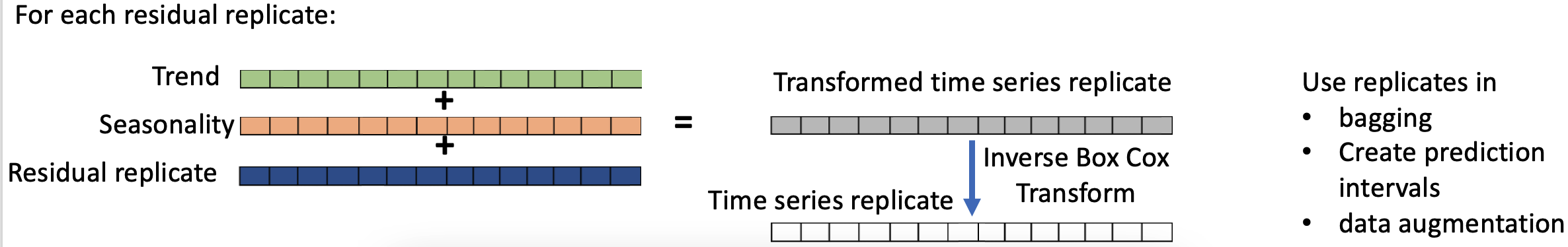
Starting with a given seasonal time series in the upper left of the diagram, we will perform a Box-Cox transform, followed by a STL decomposition. With the residuals resulting from the STL decomposition, replicate residuals will be formed and which are highlighted in a yellow box in the diagram. These replicate residuals are created by using the moving_block_bootstrap() function from pyredraw.

With each of the bootsrapped residual replicates, we will then add back the trend and seasonality time series components found from the STL decomposition, and perform an inverse Box-Cox transform to obtain a bootstrapped replicate of the original time series.
Import packages, time series data, and create a Numpy array
import pandas as pd
import numpy as np
from scipy.stats import boxcox
from scipy.special import inv_boxcox
from statsmodels.tsa.seasonal import STL
import matplotlib.pyplot as plt
from pyredraw.ts import moving_block_bootstrap
from pyredraw.plotting import plot_replicates
# read in time series data
df = pd.read_csv("iceland_montly_retail_debit_card_expenditures.csv",
                  index_col='date',
                  parse_dates=True
                 )
df.head()
| monthly_expenditure | |
|---|---|
| date | |
| 2000-01-01 | 7.204 |
| 2000-02-01 | 7.335 |
| 2000-03-01 | 7.812 |
| 2000-04-01 | 7.413 |
| 2000-05-01 | 9.136 |
# create pandas series, add frequency of time index (Monthly, Starting)
sr = df.squeeze()
sr = sr.asfreq('MS')
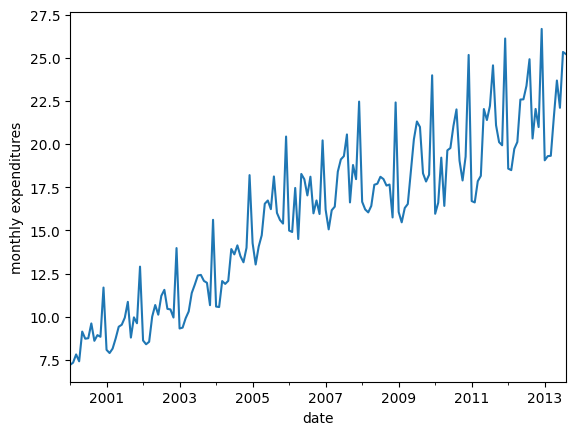
# plot time series - time series shows clear seasonality
ax = sr.plot()
ax.set_ylabel("monthly expenditures")
plt.show()
sr.values
array([ 7.204,  7.335,  7.812,  7.413,  9.136,  8.725,  8.751,  9.609,
        8.601,  8.93 ,  8.835, 11.688,  8.078,  7.892,  8.151,  8.738,
        9.416,  9.533,  9.943, 10.859,  8.789,  9.96 ,  9.619, 12.9  ,
        8.62 ,  8.401,  8.546, 10.004, 10.675, 10.115, 11.206, 11.555,
       10.453, 10.421,  9.95 , 13.975,  9.315,  9.366,  9.91 , 10.302,
       11.371, 11.857, 12.387, 12.421, 12.073, 11.963, 10.666, 15.613,
       10.586, 10.558, 12.064, 11.899, 12.077, 13.918, 13.611, 14.132,
       13.509, 13.152, 13.993, 18.203, 14.262, 13.024, 14.062, 14.718,
       16.544, 16.732, 16.23 , 18.126, 16.016, 15.601, 15.394, 20.439,
       14.991, 14.908, 17.459, 14.501, 18.271, 17.963, 17.026, 18.111,
       15.989, 16.735, 15.949, 20.216, 16.198, 15.06 , 16.168, 16.376,
       18.403, 19.113, 19.303, 20.56 , 16.621, 18.788, 17.97 , 22.464,
       16.658, 16.214, 16.043, 16.418, 17.644, 17.705, 18.107, 17.975,
       17.598, 17.658, 15.75 , 22.414, 16.065, 15.467, 16.297, 16.53 ,
       18.41 , 20.274, 21.311, 20.991, 18.305, 17.832, 18.223, 23.987,
       15.964, 16.606, 19.216, 16.419, 19.638, 19.773, 21.052, 22.011,
       19.039, 17.893, 19.276, 25.167, 16.699, 16.619, 17.851, 18.16 ,
       22.032, 21.395, 22.217, 24.565, 21.095, 20.114, 19.931, 26.12 ,
       18.58 , 18.492, 19.724, 20.123, 22.582, 22.595, 23.379, 24.92 ,
       20.325, 22.038, 20.988, 26.675, 19.061, 19.303, 19.323, 21.573,
       23.685, 22.104, 25.34 , 25.211])
Perform Box-Cox transform and STL decomposition on transformed result
# Do box-cox transform
boxcox_array, lambda_val = boxcox(sr.values)

# make series from array resulting from box-cox
boxcox_series = pd.Series(
    boxcox_array, index=pd.date_range("1-1-2000", periods=len(boxcox_array), freq="MS")
    , name="monthly_expenditures"
)
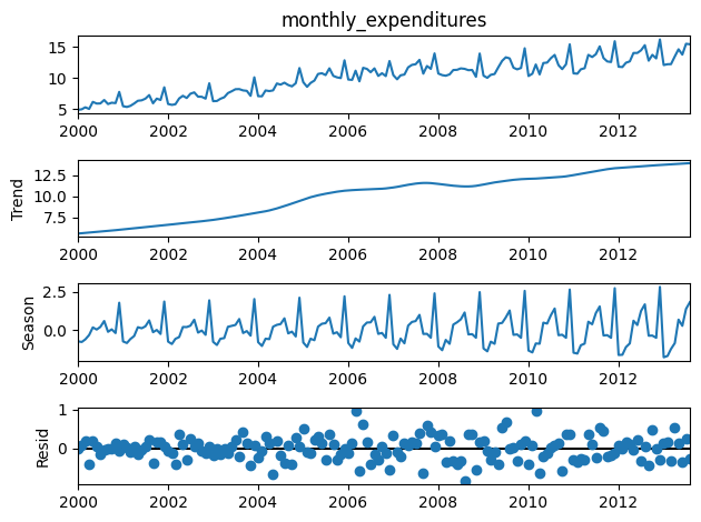
# do STL decomp (note seasonal = period+1, seasonal must be odd)
period=12
stl = STL(boxcox_series, seasonal=(period+1))
stl_result = stl.fit()

# Plot STL decomposition results
fig = stl_result.plot()
Apply moving_block_bootstrap from the pyredraw package to STL residuals
# define parameters for moving block bootstrap
block_length = int(2 * period)
number_replicates = 10

# do moving block bootstrap of STL residuals
residual_replicates = moving_block_bootstrap(stl_result.resid,
                                             block_length,
                                             number_replicates,
                                             seed = 1027)
residual_replicates.shape
(10, 164)
# make residual array into pandas dataframe
# adding back seasonal and trend from STL, do inverse Box-Cox
df_replicates = pd.DataFrame(columns=["monthly_expenditures", "replicate"])
number_replicates, _ = residual_replicates.shape
number_replicates_array = np.arange(0, number_replicates)

for replicate in number_replicates_array:
    # make residual in a pandas series with correct datetime index
    sr_temp = pd.Series(residual_replicates[replicate,],
                        index=pd.date_range("1-1-2000",
                                            periods=len(residual_replicates[replicate,]),
                                            freq="MS"),
                         name="monthly_expenditures"
                        )
    # add seasonal and trend components from STL to residual replicate
    sr_total_temp = sr_temp + stl_result.seasonal + stl_result.trend
    sr_total_temp =sr_total_temp.rename("monthly_expenditures")

    # do inverse Box-Cox (using exponent lambda that was found in the initial Box Cox)
    sr_inv_boxcox = inv_boxcox(sr_total_temp, lambda_val)

    # make pandas series into temp dataframe and add replicate field
    df_temp = pd.DataFrame(sr_inv_boxcox)
    df_temp["replicate"] = replicate

    # concatenate
    df_replicates = pd.concat([df_replicates, df_temp])
df_replicates.info()
df_replicates.head()
<class 'pandas.core.frame.DataFrame'>
DatetimeIndex: 1640 entries, 2000-01-01 to 2013-08-01
Data columns (total 2 columns):
 #   Column                Non-Null Count  Dtype
---  ------                --------------  -----
 0   monthly_expenditures  1640 non-null   float64
 1   replicate             1640 non-null   object
dtypes: float64(1), object(1)
memory usage: 38.4+ KB
| monthly_expenditures | replicate | |
|---|---|---|
| 2000-01-01 | 6.639942 | 0 |
| 2000-02-01 | 6.726259 | 0 |
| 2000-03-01 | 6.302820 | 0 |
| 2000-04-01 | 8.579374 | 0 |
| 2000-05-01 | 9.398532 | 0 |
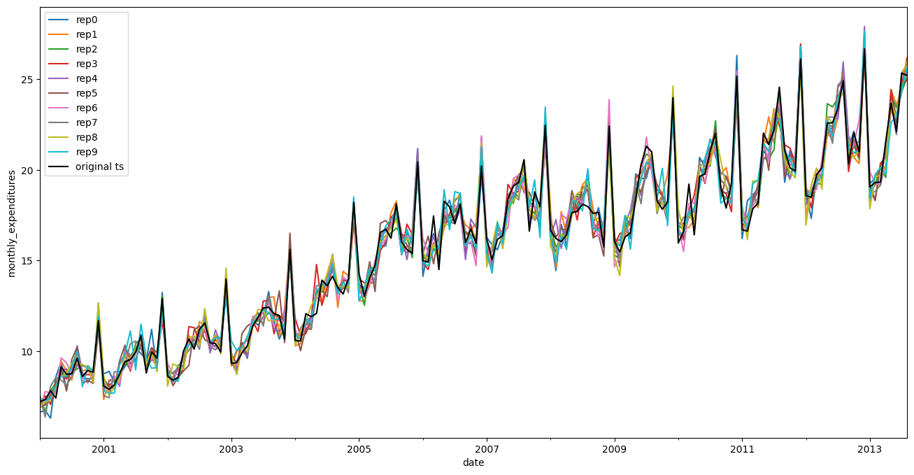
Plot replicates and original time series on same axis to compare
# Plot replicates and original time series
plot_replicates(sr, df_replicates, "monthly_expenditures")
Citation:
C. Bergmeir, R. J. Hyndman, and J. M. Ben´ıtez, “Bagging exponential smoothing methods using STL decomposition and Box–Cox transformation,” International journal of forecasting, vol. 32, no. 2, pp. 303–312, 2016.